
Analyze and Visualize with CATMA
Tutorial 2
A German version of this tutorial with Franz Kafka’s Erstes Leid as sample text can be found here: Jan Horstmann (2019): Analyse und Visualisierung mit CATMA. In: forTEXT. Literatur digital erforschen. https://fortext.net/routinen/lerneinheiten/analyse-und-visualisierung-mit-catma [accessed: December 9, 2019].
Key Data
- Object of investigation: Edgar Allan Poe’s The Tell-Tale Heart (1843)
- Methods: analysis, visualization, semi-automatic annotation
- Goals: quantitative analysis of text and annotation data; creation of queries and interactive visualizations; modification of visualizations; automatic annotation of selected keywords
- Duration: approx. 90 minutes
- Level of difficulty: easy
Components
- Application Example
Which text and annotations will you explore?—Here you will learn how to analyze Poe’s short story The Tell-Tale Heart and visualize analysis results. - Preliminary Work
What do you need to do before the analysis?—Here you will get information about necessary preliminary work. - Functions
Which functions can you use in CATMA’s Analyze module?—Get to know the individual components of the module and solve sample tasks. - Solutions to the Sample Tasks
Have you solved the sample tasks correctly?—Here you will find answers.
Application Example
This tutorial shows you how to analyze and visualize textual data with CATMA. In part, you will build on the work done in the tutorial → Manual Annotation: you will analyze and visualize textual data from Poe’s short story The Tell-Tale Heart (1843) in addition to the annotations on the narrator’s style and attitude that you created previously. (You can still perform most of the functions and tasks described here even if you did not create manual annotations previously.
Preliminary Work
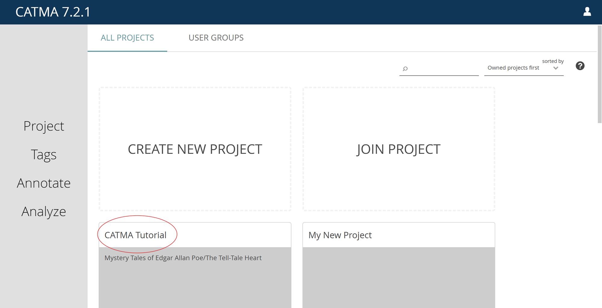
In order to work with this tutorial, you must have completed at least the section “Preliminary Work” from the first tutorial → Manual Annotation. In that section, you learned how to register for a CATMA account, create a project and upload the text that you want to investigate. The section “Functions” from the first tutorial is optional. If you did not complete it in advance, you can still follow this tutorial at large. To use the functions of the Analyze module in CATMA, go to https://app.catma.de and log in. On the next page (see Fig. 1), CATMA’s dashboard, you should find the project created in the first tutorial (we called it “CATMA Tutorial” there). Open the project by clicking on the tile.
Functions
CATMA supports hermeneutic text investigation by integrating text annotation and analysis into a cyclical, iterative workflow. Typically you will combine your work in the Annotate module with the features offered by the Analyze module. While you practice close reading when annotating, the Analyze module supports a distant reading approach: you can investigate your texts, even without reading them.
There are two ways to reach the Analyze module from the Projects module:
- You can open the text by double-clicking it. Once you are in the Annotate module, click the ANALYZE button below the text (this way the text together with all associated annotation collections will be pre-selected in the Analyze module).
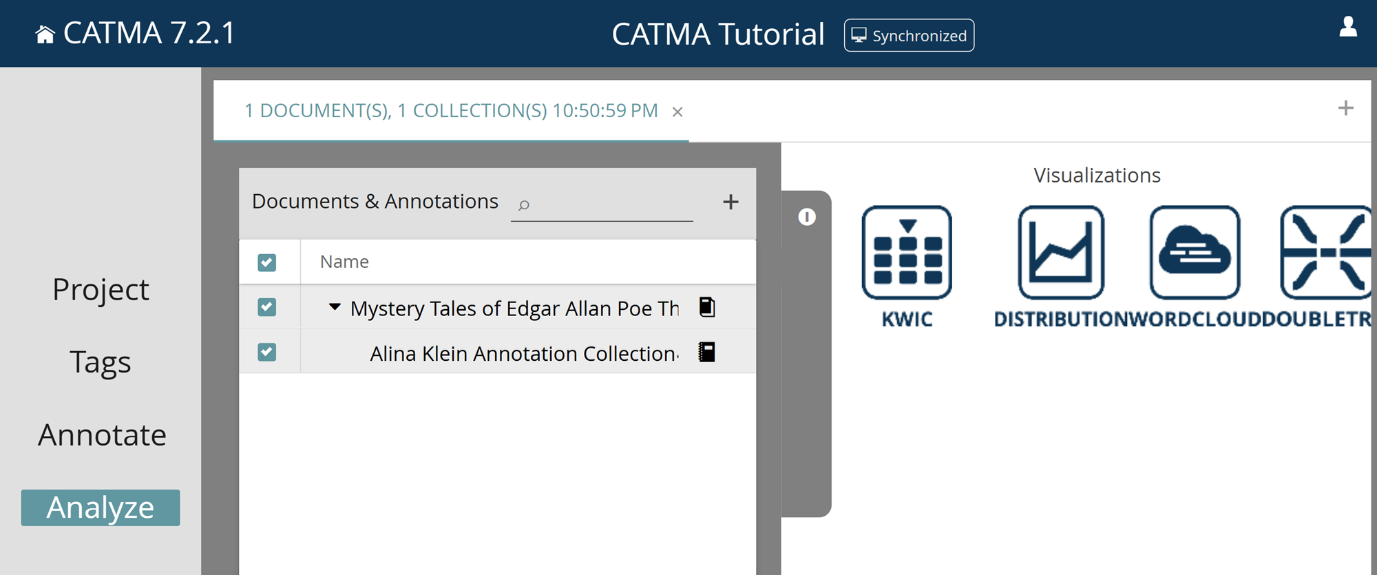
- Alternatively, you can directly click on Analyze in the navigation bar on the left. In the gray drawer that opens automatically, you have to select the texts and annotation collections you want to analyze (see Fig. 2). Select both the text and your annotation collection (you can also select all resources at once by clicking in the upper box next to Name).
What does it mean to select texts and annotation collections for analysis? The Analyze module performs quantitative operations. These can be based on either text-only data (such as word frequencies or distributions) or on annotation data that you created yourself (such as tag frequencies or distributions). CATMA also offers the possibility to create complex queries, i.e. a combination of several searches, that can, for example, be based on both text and annotation data.
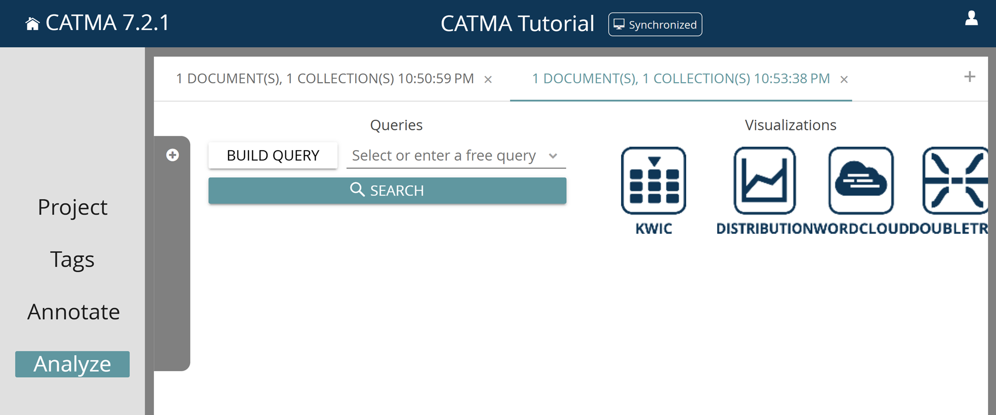
Whenever you add or delete one or more annotations in the Annotate module, you are modifying the annotation data, meaning that you will potentially get different results in the Analyze module. You can open a new analysis tab using the small plus icon in the upper right corner of the Analyze module in order to, for example, integrate further annotation collections into the analysis. Similarly, whenever you click on the ANALYZE button in the Annotate module again, a new tab will open in the Analyze module to keep the different analysis sessions separate (as different texts and annotation collections may have been selected). The tabs have a timestamp so that you can keep track of the chronological order of analysis sessions (see Fig. 3).
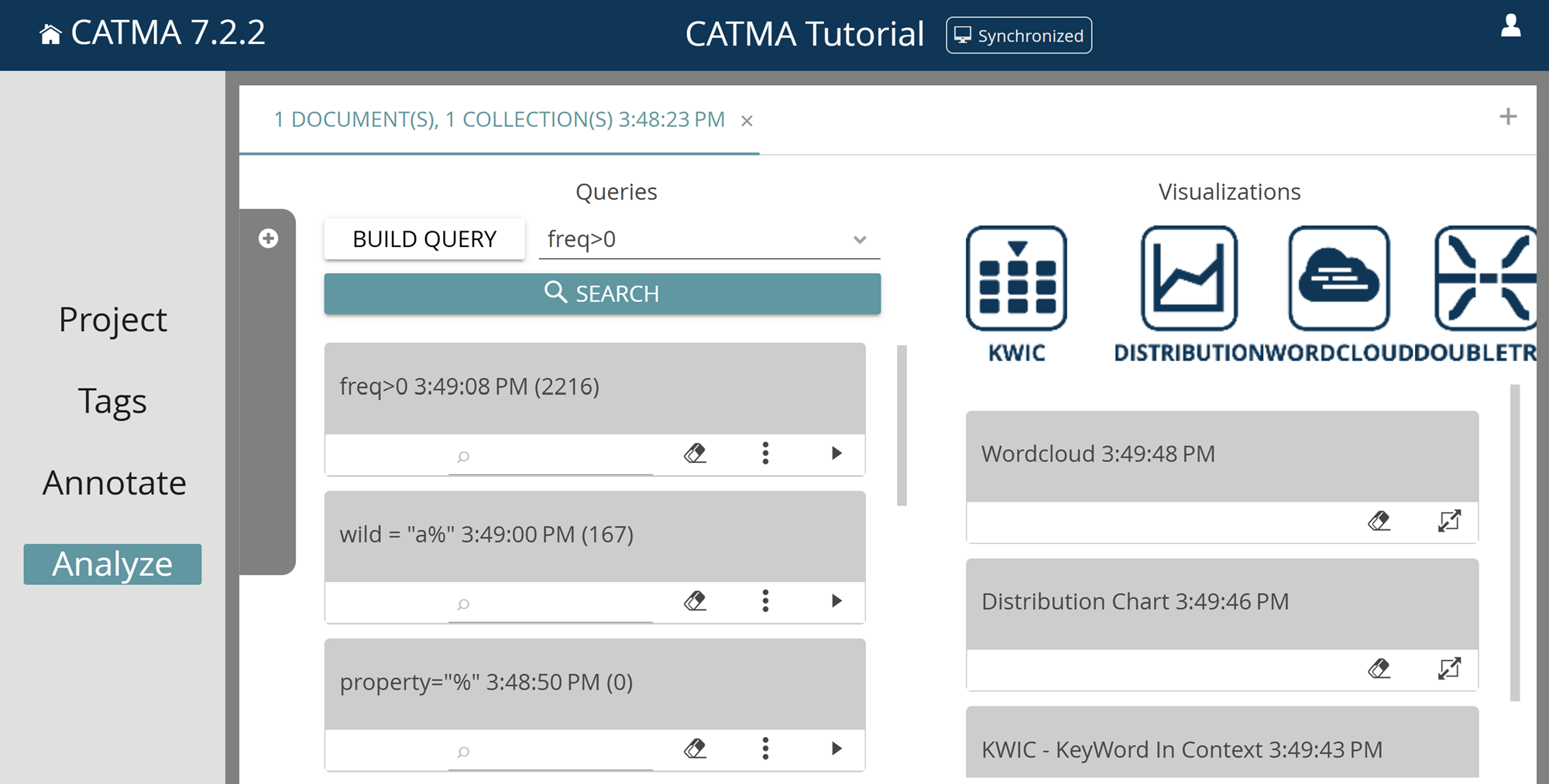
If you look at the structure of the Analyze module, you will see that it is generally divided into two areas: Queries on the left and Visualizations on the right. A query defines which information is retrieved from the text and/or annotation data. You can view, explore and process the results of the query in various interactive visualizations. Text visualization is thus understood as an integral part of text analysis.
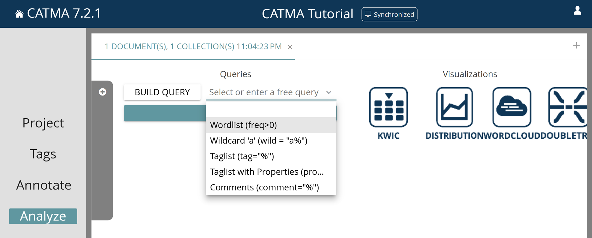
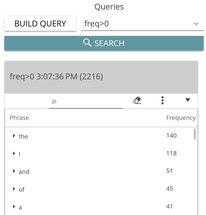
For the simplest tasks, CATMA offers you a few predefined queries. Click on the small arrow pointing downwards next to “Select or enter a free query” and select the first option: Wordlist (freq>0) (see Fig. 4). This action gives you a list of all words in the text, sorted by frequency (see Fig. 5). By the way: the technical expression “freq>0” in the brackets after “Wordlist” is the query language expression for the task of showing all words with a frequency above zero.
Task 1
How many words does Poe’s story contain? What is the most common content word (= a word with “more” semantic meaning than function words such as articles, pronouns etc.)? What else do you notice about the given “words”? And what would the query be that returns all words in the text that occur more than five times?
If you have entered another query to search for all words occurring more than five times, you will have noticed that the result of this query is displayed above the previously created wordlist. It is generally possible to perform several queries one after the other and collect the result lists in this form. Each query result has a small search field in the header to quickly search the respective list (see Fig. 6). You can delete a result list by clicking on the small eraser icon. The three-dot menu to the right contains different view options, as well as options to export your query results in CSV format. The arrow icon allows you to expand and collapse the result lists in order to have a better overview of all your queries.
Word frequencies can also be explored visually in the form of a wordcloud. This is one of the visualization possibilities for query results currently implemented in CATMA. To create a visualization, run a query (such as freq>0) and then click on the desired icon on the right; in this case Wordcloud.
The wordcloud view opens and on the left you will see the query result list again. (If you have multiple result lists, you can choose between them at the top left of the currently displayed list.) From this list you can now select the words to be displayed in the wordcloud by using the down arrows in the “Select” column. The selected words are moved into a second list below, and everything in this list is fed into the visualization.
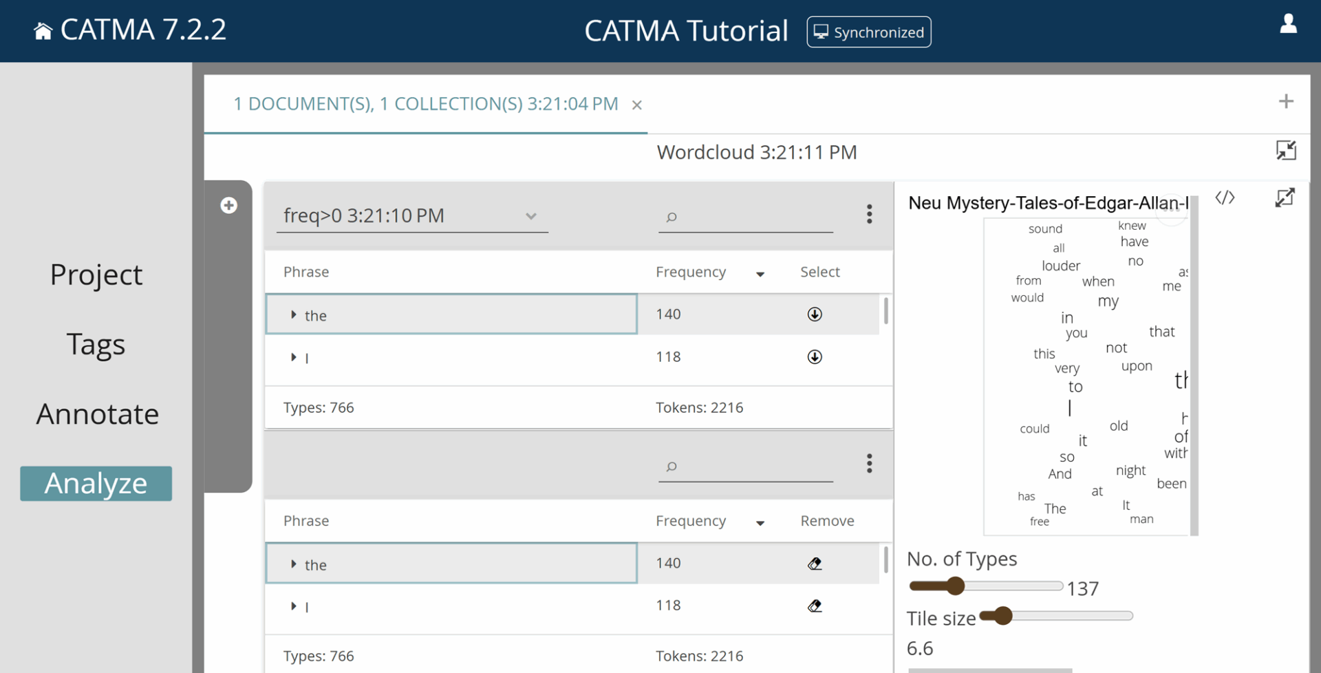
This way, you can manually compile a list of words that should appear in the wordcloud. Hint: The “Select all” option available via the three-dot menu of the query result list integrates all words into the wordcloud. You will see a wordcloud in which the size of the words represents their frequency in the text (see Fig. 8). The second list, that you created by selecting some or all entries from the first, allows you to delete individual values (such as punctuation marks, numbers, or words belonging to possible paratexts) using the eraser icon, so that they also disappear from the visualization.
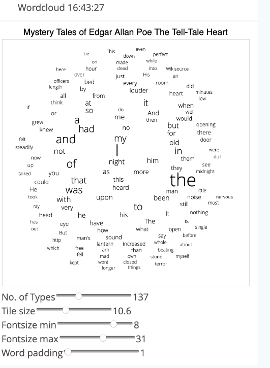
Under the wordcloud, you can manipulate your visualization using the different sliders. You can change the maximum number of words (types) included in the visualization, the size of the wordcloud, as well as the font size and distance between the individual words (Word padding).
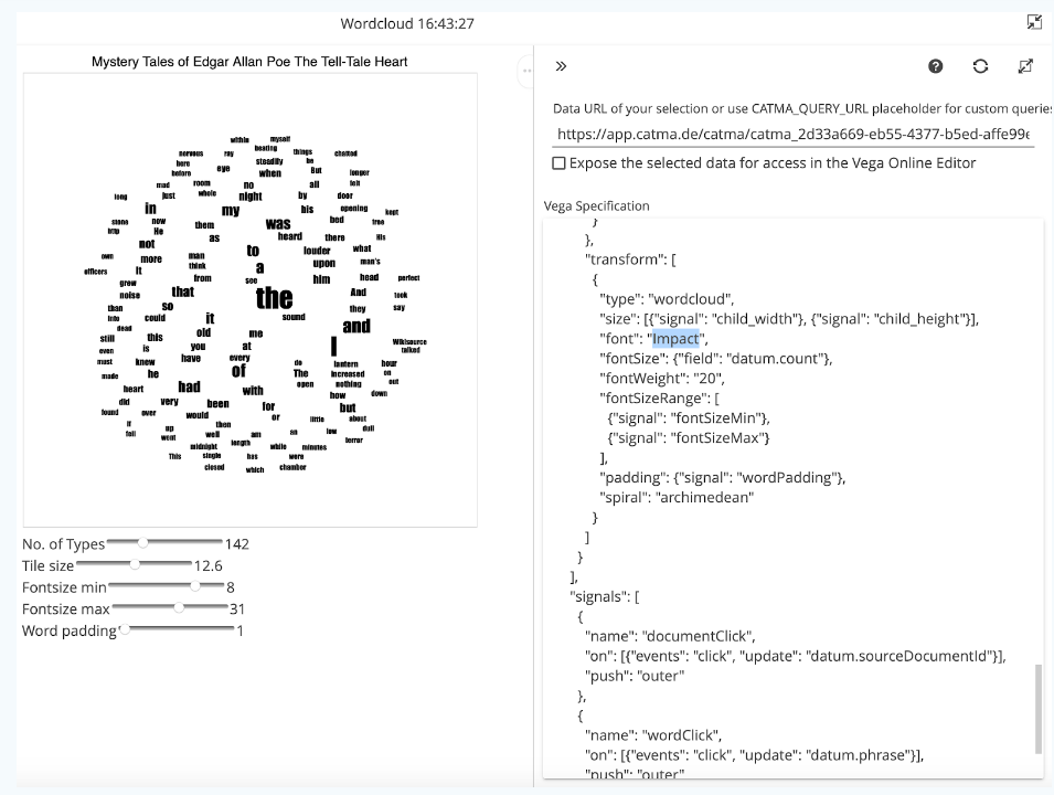
Side note: All visualizations in CATMA have dot menus in the upper right corner that allow you to export your visualization as an image (PNG) or vector (SVG) file. You can also view the source code of each visualization here. CATMA visualizations are based on the Vega visualization language. With some practice, Vega allows you to create any (even interactive) visualization that fits your data. You could open the Vega Editor, potentially create a completely new visualization based on selected query results and load the code of this new visualization back into your CATMA project. In this introductory session, however, we will skip these expert functions. To make smaller adjustments, it is easier to click on the small button to the right of the three dots. The visualization code appears in a column on the right: manipulations in this code (after a click on the refresh icon above) will change the displayed visualization. Why don’t you try to change the font as shown in Fig. 8 for example?
To close a visualization and return to the Analyze module, click on the icon with the two arrows pointing to each other at the top right. The visualization is minimized and kept in the visualization area of the Analyze module, much like the query results (see Figure 10). From here, you can return to individual visualizations at a later point.
Now let’s turn back to the queries. Among the predefined queries, you will find the word list, a tag list (optionally including properties), comments and the option Wildcard. With the wildcard option you can search for word beginnings, for example. “Wildcard” stands for placeholders (these are the “%” symbols in CATMA’s query language). The suggested wildcard query “a%” will therefore show you all words that begin with a small “a”.
Task 2
How many words in Poe’s story begin with the letter “a”, how many with “b”?
Especially for beginners, CATMA provides the BUILD QUERY feature, which uses common language questions to help you compose your query. After each run through BUILD QUERY, the created query appears at the top of the Analyze module. Paying attention to the form of these queries allows you to quickly learn CATMA’s query language. You can find a systematic overview of CATMA’s query language here.
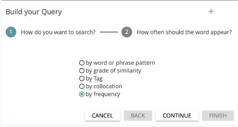
In this tutorial, you will now use the BUILD QUERY feature. If you click on the corresponding button, you will first be asked what you want to search for (see Fig. 11): words or phrases, similarities, tags, collocations or frequencies. First select by frequency and then click on CONTINUE.
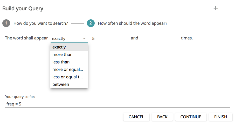
In the next step, you can specify which words should be displayed: all words that appear “exactly” x times in the text, all words that appear more or less than x times (“more than” and “less than”), “more or equal than” or “less or equal than” x times, or “between” x and y times (see Fig. 12). You set the numerical values yourself. At the bottom of the dialog, you can already see what the query will look like. Complete the query by clicking on FINISH.
Task 3
How many words occur five or more times, but less than 16 times? What does the query look like? Which physical senses seem to be predominant in the story?
This way, you can now build a large number of queries without having to know the query language. (If you want to analyze a text or a corpus with many queries, however, we recommend that you learn the rather simple language—you will quickly save a lot of time. Additionally, not all of the more complex queries can be created using BUILD QUERY). Now click your way through the other BUILD QUERY functions (except by tag) and try to answer the following questions.
Task 4
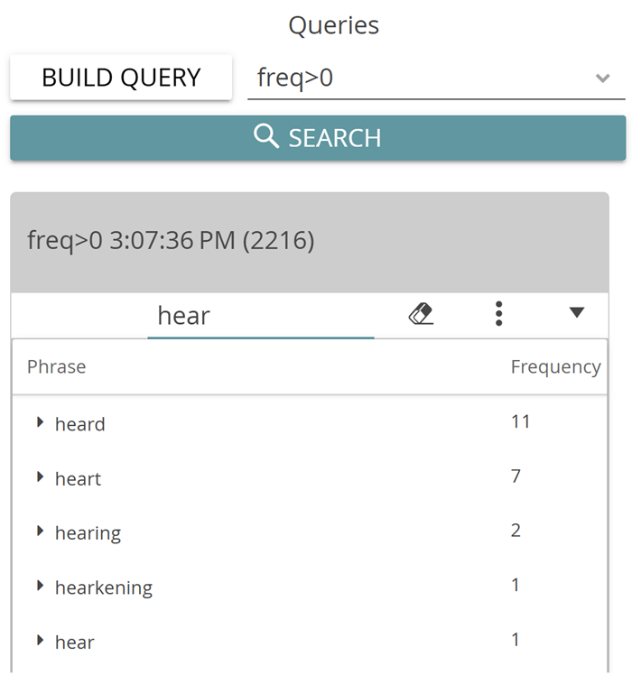
How many words have a 70% similarity to “heart”? Use the “by grade of similarity” query option. Increase the similarity to 80%. Do it again with 85%. And how often does the word “mad” appear near the word “me” (within a span of ten words)? Use the “collocation” function for this. What do the respective queries look like?
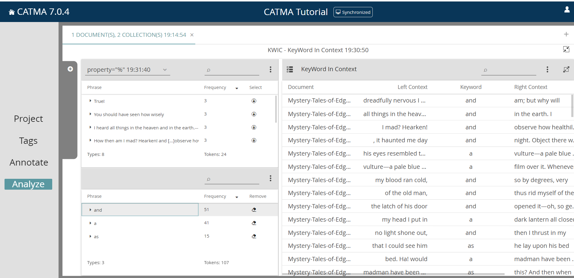
CATMA offers two visualization options for examining word contexts: KWIC (KeyWord In Context) and DoubleTree. Both visualization types can display selected words in their respective contexts; KWIC does this in the form of a table that displays a selectable number of words that precede and follow the selected word. This contextualizing exploration of selected words enables a selective and efficient insight into semantic constellations. To display a keyword in its context, first create a word list again and then click on the KWIC icon on the right; you will be taken to the KWIC visualization view. Here you can select words from the list at the top left (like you did before) and thus compile another list of selected keywords at the bottom left. On the right side, each occurrence of the chosen keyword appears in a table with its respective context (see Fig. 13). Further selected keywords are added to this table; you can remove keywords by clicking on the eraser icon in the list at the bottom left. To change the KWIC context size, click on the three-dot menu of the KWIC table and click on Edit Context Size. Now you can select how many words, from 1 to 30, should be displayed that precede and follow the selected words. You can resize the individual columns of the keyword list with your mouse (this generally applies to most columns, panels, dialogs etc. in CATMA) or change the ordering of the rows by clicking on the column headings. Try it now by clicking on Start Point, which will change the default ordering of ascending by start point to descending, i.e. to reverse order of appearance in the text. By the way, the Start Point and End Point numbers are the so-called character offsets, i.e. the index of the first and last letters of the occurrence of the selected word in the text, respectively. For a keyword with five letters, the End Point will thus always be exactly five more than the Start Point.
If you find a passage in the KWIC table that seems interesting to you or for which you need more context, you can always jump directly from this list to the corresponding text passage in the Annotate module by simply double-clicking the row in the KWIC table that interests you. The relevant keyword (token) is then underlined with a red and yellow bar in the text. A click on Analyze in the navigation bar on the left takes you back to the list. To avoid having to constantly switch between Analyze and Annotate, the KWIC table is also shown in the Annotate module.
Task 5
Analyze the word “I” in its contexts using the KWIC visualization. What do you notice?
The DoubleTree visualization provides a more interactive form of context exploration. Close the KWIC visualization by clicking on the arrow icon in the upper right corner and then click on the DOUBLETREE icon. The creation of the visualization works according to the known scheme: select the desired keyword on the left, which is then visualized on the right as a DoubleTree (see Fig. 14). The difference is that only one keyword is displayed at a time — another one can be selected by clicking on it in the bottom left list.
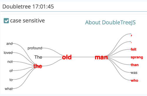
Initially, you will see the selected keyword highlighted in red and displayed only once in the middle of the DoubleTree. The various adjacent words are displayed to the left and to the right. If a word occurs frequently in the context of the keyword, it is displayed larger than if it occurs less frequently. If you click on one of the adjacent words, the further context unfolds (by the way, you can freely move the DoubleTree on the screen with your mouse). The word that was clicked will turn red, too, as will those words that occur in the same context but on the opposite side of the initially selected keyword. This offers you a possibility to reflect upon the sentence structure. The DoubleTree visualization thus provides a structured overview of the way vocabulary is used in a specific text, and offers, for example, the possibility to draw conclusions about characterizations. For this visualization, the case sensitivity common in CATMA can be switched off, i.e. upper and lower case word variants can be combined.
Task 6
Explore the contexts of the word “man” with the DoubleTree visualization. Can you say anything about the characterization of the character? Try the same with “I”.
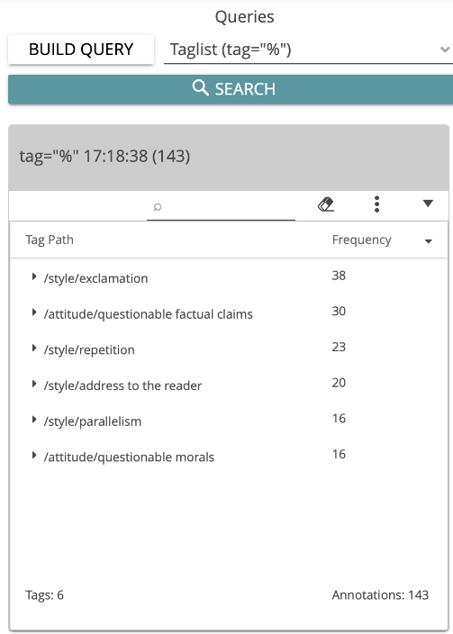
Now, how can the annotations created in the previous tutorial be examined in the Analyze module? (If you haven’t completed the tutorial → Manual Annotation, you can jump to the paragraph after figure 15 below). Close the DoubleTree visualization. You can generate the entire list of all tags assigned in the annotation process using the predefined query Taglist (tag=”%”). The annotated phrases are displayed by default. If you want to organize the results by tag category instead, select “Group by Tag Path” from the three-dot menu. In the result, you can see which tag was assigned how often (see Fig. 15).
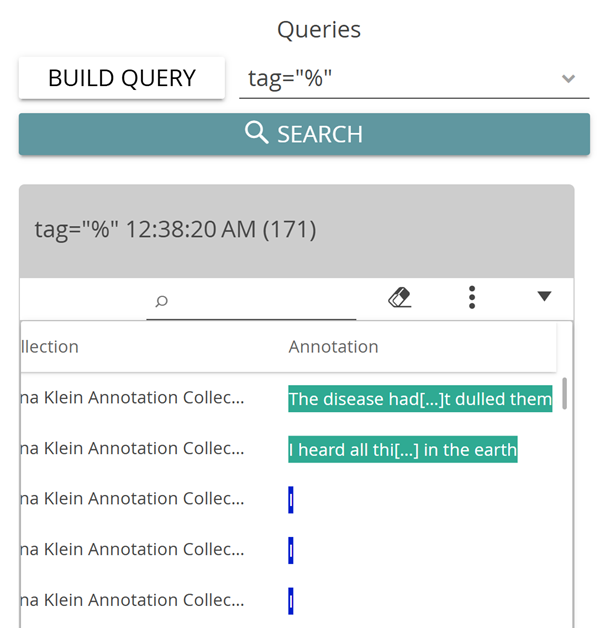
You can also display the specific annotations and properties using the options “Display Annotations as Flat Table” or “Display Properties as Columns” (see Fig. 16).
You have the possibility to generate distribution graphs for words or tags—the fourth visualization option in CATMA. These distribution charts are created in the same way as the other visualizations, i.e. by transferring individual lines from the query results to a visualization-specific second list, which in turn can be manipulated to modify the visualization. In this case, we want to see the distribution for assigned tags. (If you did not create any annotations, simply create a wordlist and select individual words for the distribution visualization.)
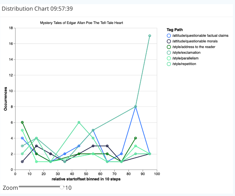
Build a tag list as before and select the option “Group by Tag Path” in the three-dot menu. Then click on the DISTRIBUTION icon on the right. Now choose “Select All” in the three-dot menu of the query result to transfer all lines into the visualization list. A line chart appears on the right, showing the distributions of the tags you have assigned (see Fig. 17). The x-axis refers to the entire text length, which is divided into 10% segments here (based on the number of letters). The number of occurrences per segment appears on the y-axis. You can enlarge the entire visualization using the zoom slider.
Task 7
Create a distribution chart for the tags you assigned. What do you find noteworthy? What purpose is this form of visualization suitable for? In which respect would another visualization be more useful?
You can also use BUILD QUERY to search for individual tags. To do so, select the option by tag in step 1. After a click on CONTINUE the tagset appears, from which you can select the desired (sub)tag. A corresponding query could look like this: tag=”/attitude/questionable morals%”.
As another example, the query tag=”/style%” looks for all annotations of the four subtags belonging to the parent tag “style” in the tagset that we created in the first tutorial (i.e. the subtags “address to the reader”, “exclamation”, “parallelism” and “repetition”).
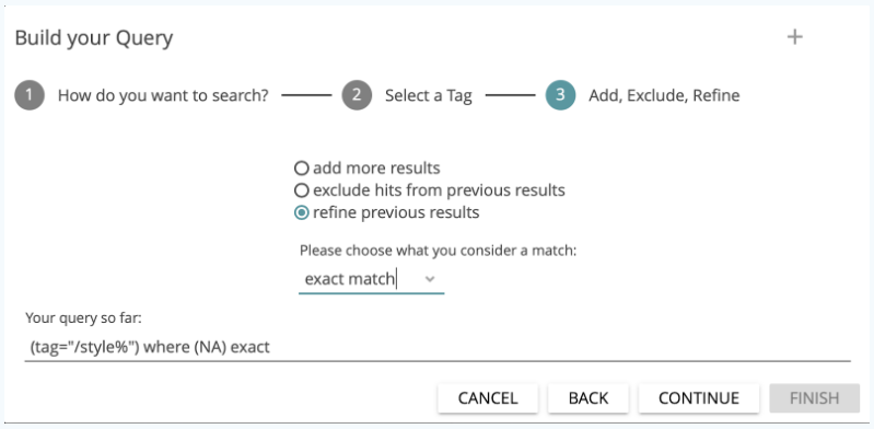
It is also possible to generate complex queries by clicking CONTINUE instead of FINISH at step 2 of the wizard interface. You will then be asked if you want to “add more results”, “exclude hits from previous results”, or “refine previous results”. For the latter two, you must also determine the type of relationship between previous results (i.e. the query results so far) and the results from the exclusion or refinement expression that you are adding. The options are “exact match”, “boundary match” and “overlap match” (see Fig. 18). The “exact match” option matches when the two query components apply to the exact same string of characters (e.g. two annotations, using different tags, that overlap exactly). With “boundary match”, any occurrence of your query’s first component that lies completely inside the boundaries of the second component will be returned (e.g. all annotations using one a tag that are enclosed by annotations using another tag). Finally, the third and most permissive option (“overlap match”) allows you to find partial overlaps (such as annotations using different tags that overlap each other, or overlapping words/phrases and annotations).
For further explanation and examples, please see the documentation for CATMA’s query language here.
Task 8
Search for all incidents in which words beginning with “hear” overlap with the annotations of questionable factual claims. What does the query look like? How many results do you get?
The last function of the Analyze module that we want to approach in this tutorial is that of semi-automatic annotation. You may have noticed by chance that the wordcloud and distribution chart visualizations that you generated in CATMA are interactive, i.e. you can click on individual areas in the visualizations and get more options. We will try this out with a simple wordcloud visualization of all words in the text.
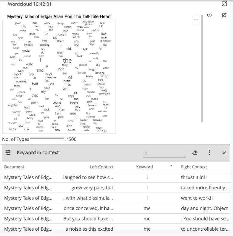
Open the previously created wordcloud visualization again and add all words (if this is not still the case). If you have closed the respective Analyze tab in the meantime, create a new word list, click on “Wordcloud”, select all results using the corresponding option in the three-dot menu and increase the number of displayed words (types) using the slider. If you now click on individual words in the wordcloud, a KWIC table opens below the visualization (see Fig. 19). Do this with the words “I”, “me”, “my” and “myself”.
With KWIC tables in CATMA, annotations can generally be created semi-automatically for selected keywords. To do this, click on the selection icon to the left of the heading “KeyWord In Context” and select all rows by checking the top box next to the “Document” column heading. Alternatively, you can select individual rows from the list. After having made a selection, click on you the option “Annotate Selected Rows” in the three-dot menu.
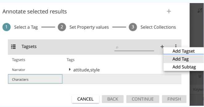
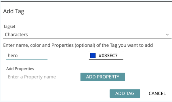
A dialog window opens (see Fig. 20), which allows you to either select existing tags or to create new tagsets and tags to be used for semi-automatic annotation. Now create a tagset named “Characters” and, in this tagset, the tag “hero” (see Fig. 21). Select this new tag in the tag list and click on CONTINUE.
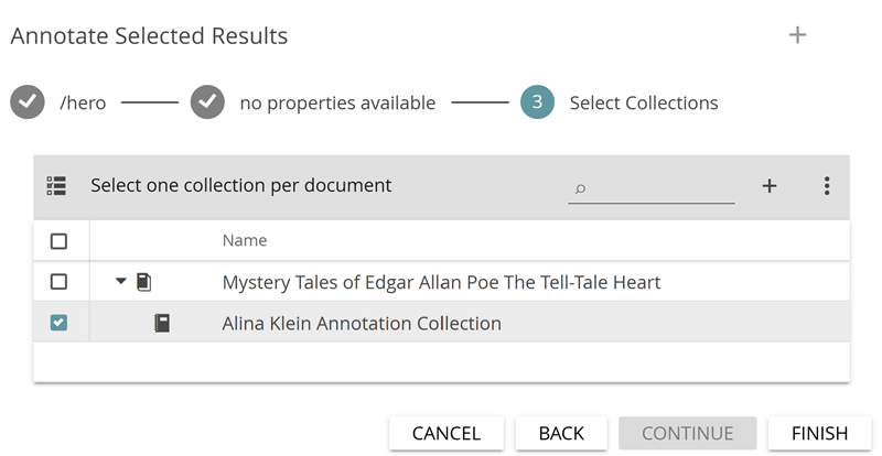
In a the step, you are asked in which annotation collection the new annotations should be stored. Select your own annotation collection (see Fig. 22) and click on FINISH. The new annotations will be created.
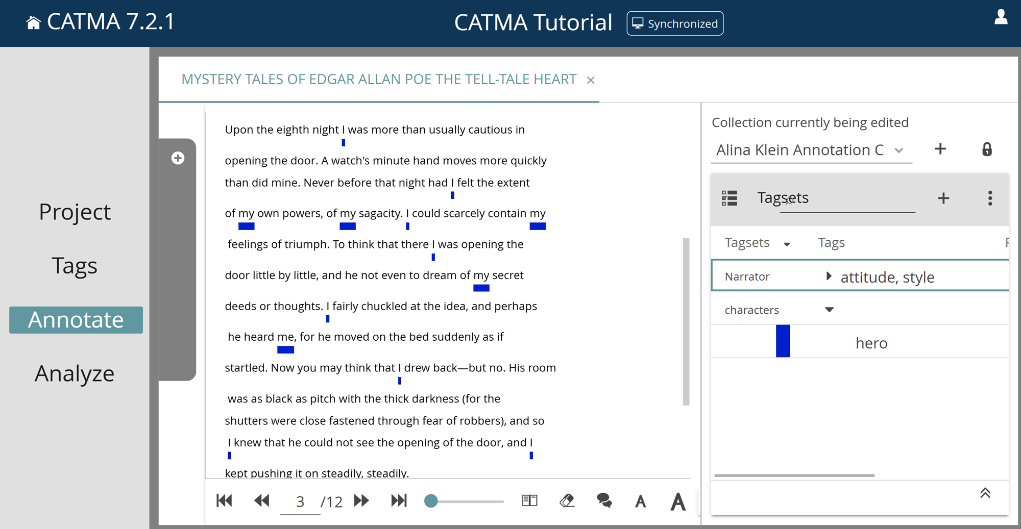
You have now annotated all selected keywords in the KWIC table with the tag “hero”. Double clicking on a row in the table will take you back to the Annotate module (see Fig. 23), where you can see the new annotations (you may first have to click on the eye symbol next to the corresponding tagset on the right, if it is crossed out).
Task 9
Choose words from the wordcloud or create a KWIC table from the usual wordlist and semi-automatically annotate them with an “opponent” tag. Which words or phrases qualify for being annotated as “opponent”? For what kind of annotation tasks is the semi-automatic annotation feature particularly suitable? In which cases is caution recommended?
You are now familiar with all the basic functions of the Analyze module in CATMA: You can create simple and complex queries, build and manipulate result lists for visualizations, modify visualizations and generate KWIC tables for semi-automatic annotation.
Task 10
Build a distribution chart containing the tags “hero” and “opponent”. What can be seen from the representation of the two tags?
Solutions to the Sample Tasks
Task 1: How many words does Poe’s story contain? What is the most common content word (= a word with “more” semantic meaning than function words, such as articles, pronouns etc.)? What else do you notice about the given “words”? And what would the query be that returns all words in the text that occur more than five times?
The overall number of wuery results is displayed in brackets in the gray header above the result list, as well as at the bottom of the list in the footer. The Tell-Tale Heart accordingly contains 2216 word occurrences (tokens) and 766 word types (unique words). But beware: the words from the paratext, which contains information about the edition, the text, its author and the editor, are counted as well. The words “Poe” or “Wikisource” therefore do not appear in the story The Tell-Tale Heart as indicated. When analyzing word frequencies, always keep an eye on how the underlying document is designed.
The word “was” appears 33 times (or, in case you do not consider pronouns function words, “I” appears 118 times). Even from this quick glance into the wordlist and without knowing the text, it is possible to infer the main characters (homodiegetic first person narrator; no females) and the relationship between narrative time and narrated time (subsequent narration) as well as an emphasis on physical senses.
Punctuation marks are also counted as “words” in CATMA (if you deactivate “Filter Punctuation” option in the three-dot menu, you can also display them in result lists). The reason for this is that a word could basically be defined by the spaces before and after the word. According to this rule, punctuation marks (usually occurring without spaces next to a word) would be counted together with the words (i.e. “interpret” and “interpret,” would be two distinct words). At the same time, one does not want to ignore the frequency of punctuation marks, as they can provide valuable impulses for the interpretation of a text (e.g. if it contains more question marks than exclamation marks, or more periods / full stops than commas, etc.).
Finally, you may have noticed that CATMA does not count uppercase and lowercase words together (e.g. “my” occurs 28 times, “My” two times), i.e. it is case sensitive, and also counts word forms separately (e.g. “see” occurs five times, “seen” two times). So if you want to find out how often a word is used in its basic form (actually a lemma), you should add all forms of the word. The search bar in the header of the query result is suitable for this (or alternatively, wildcard or regular expression queries).
The query for all words that occur more than five times in the text should be: freq>5.
Task 2: How many words in Poe’s story begin with the letter “a”, how many with “b”?
167 tokens beginning with “a” and 90 with “b” are displayed. The second query is: wild = “b%”.
Task 3: How many words occur five or more times, but less than 16 times? What does the query look like? Which physical senses seem to be predominant in the story?
70 unique words (types) appear in the text between five and 15 times (the words of the paratexts are also counted here). The query for this is: freq = 5-15. CATMA includes the words that occur five or 15 times with this expression. Especially sound but also vision are the predominant physical senses.
Task 4: How many words have a 70% similarity to “heart”? Use the “by grade of similarity” query option. Increase the similarity to 80%. Do it again with 85%. And how often does the word “mad” appear near the word “me” (within a span of ten words)? Use the “collocation” function for this. What do the respective queries look like?
Twelve words have a 70% similarity to “heart” (be aware that an instance like “heart—for” is counted as one word here), nine words with 80%. With 85%, only “heart”, “hearty”, “earth”, “hear”, “tear”, “Heart” and “HEART” are listed. The query is: simil=”heart” 70%. It is more time-saving to simply adjust the percentage in the query bar than to use the BUILD QUERY function again for each query.
The words “mad” and “me” co-occur two times within a span of ten words. The query for this is: “mad” & “me” 10.
Task 5: Analyze the word “I” in its contexts using the KWIC visualization. What do you notice?
It is noticeable that the word “I” occurs very often, so it is probably a story with a homodiegetic first-person narrator. A closer look at the KWIC table confirms this impression, because the “I” never appears in the direct speech of another character.
Task 6: Explore the contexts of the word “man” with the DoubleTree visualization. Can you say anything about the characterization of the character? Try the same with “I”.
The DoubleTree allows you to explore a word in its various contexts. For example, the man is obviously old, scared and he dies. This may lead to conclusions about the character of the man as well as his feelings to and/or his behavior towards the narrator. For the word “I” the DoubleTree is not the most suitable visualization, because it occurs so frequently. Nevertheless, one can draw conclusions about the character of the main character: he is very active, sees, moves, could, knew etc.
Task 7: Create a distribution chart for the tags you assigned. What do you find noteworthy? What purpose is this form of visualization suitable for? In which respect would another visualization be more useful?
It is noticeable that, due to the rather short text length, the 10% segments are correspondingly short, which means that in each segment only a few annotations of each category occur. Furthermore, several of the annotated categories have similar distributions; the most striking is the exclamations tag, since 17 such exclamations take place in the last 10% of the text alone.
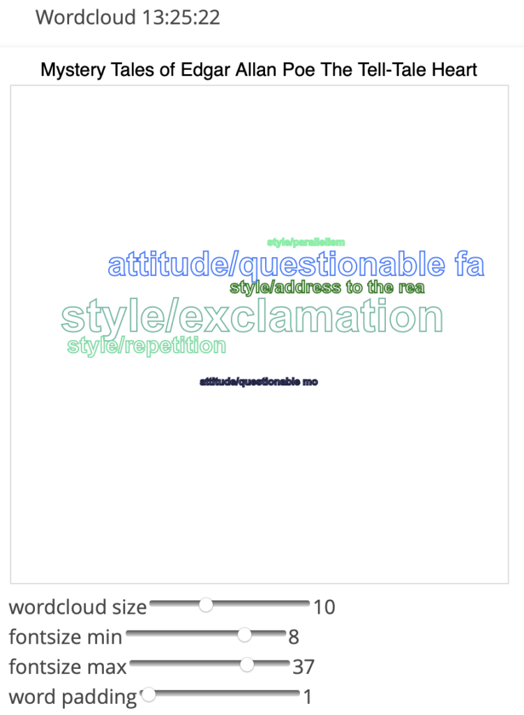
Distribution charts usually get more interesting if occurrences (e.g. between tags and certain words) are visualized and investigated. The connecting lines between the individual points of the distribution chart should also be considered critically, as they imply a continuous development. This is not usually the case in reality. Distribution charts are particularly suitable for longer texts. For a mere representation of the frequencies of assigned tags, the wordcloud is a more fitting visualization, which in this case could look somewhat like this:
Task 8: Search for all incidents in which words beginning with “hear” overlap with the annotations of questionable factual claims. What does the query look like? How many results do you get?
The query is: (wild=”hear%”) where (tag=”/attitude/questionable factual claims%”) overlap. The number of results depends somewhat on the decisions you made in the annotation process. In our case, we get nine matches (four times “heart” and three times “heard”).
Task 9: Choose words from the wordcloud or create a KWIC table from the usual wordlist and semi-automatically annotate them with an “opponent” tag. Which words or phrases qualify for being annotated as “opponent”? For what kind of annotation tasks is the semi-automatic annotation feature particularly suitable? In which cases is caution recommended?
Words/phrases like “old man”, “eye”, “heart”, “corpse”, “he”, “him”, “his”, “body”, “police”, “officers”, “they”, “them”, “their” etc. qualify to be annotated with the “opponent” tag.
Semi-automatic annotation is especially useful for the annotation of named entities (like the main character in our example). But also time forms of verbs could be annotated semi-automatically with the corresponding tags (e.g. “past”, “present”, “future” or also “simple past”, “present perfect”, “simple present”, “future I” etc.). Be careful here because there are words which can be verbs in a certain time form as well as other types of words depending on the context. The tag “hero” could also lead to difficulties in narratives with a homodiegetic narrator: here the “I” does not always have to stand for the narrator, since it can refer to every other character in direct speech. The context in the KWIC table should therefore be taken into account, especially during semi-automatic annotation.
Task 10: Build a distribution chart containing the tags “hero” and “opponent”. What can be seen from the representation of the two tags?
The distribution of the hero and opponent annotations could look somewhat like this:
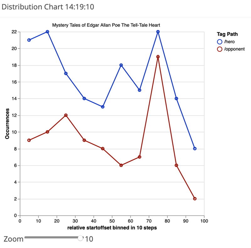
By clicking on the individual dots, you can examine single passages of the story in a KWIC table. Considering the rather parallel distribution of the two categories, it is noticeable that the curves drift apart in the section between 50 and 60%. Examining the contexts of this passage, one finds out that this is exactly the point where the “hero” kills his “opponent”, the old man. The mere distribution of frequencies thus hints to this central and important passage of the narrative.